Visualization
The figure is produced through linking the points. Therefore, in order to produce the figure, we first need to grap the axis of each point. In MATLAB, we can produce figures with two or three dimensions.
Plot with two dimensions
In Matlab, we use plot, ezplot and fplot function to produce two dimensional plot.
plot
Produce the figure for using red line and produce the figure for
using green dash line.
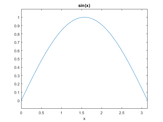
ezplot
Produce the figure for with interval of [0, pi] using
ezplot
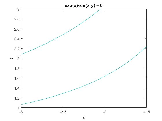
ezplot can also be used to produce figure for parametric equation and implicit function. For example, produce figure for parametric equation and
with the interval of
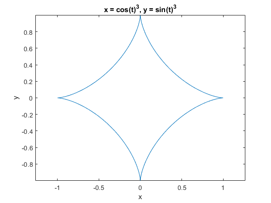
Produce figure for implicit function with the interval of
and
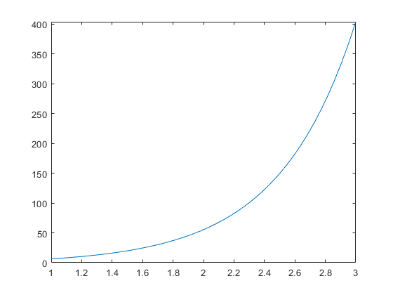
fplot
fplot('fun', lims) can be used to draw the figure in the interval lims=[xmin, xmax]. fun must be the name of the m file. fplot can not be used to produce figures for parametric equation and implicit function, but it can do multiple plotting.
Produce a figure for with the interval of
.
Open a new Matlab script fun.m and type the following;
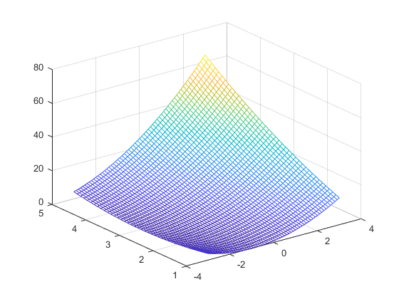
Plot with three dimensions
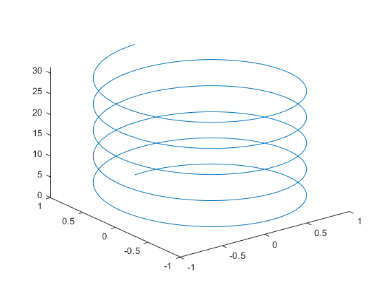
plot3(X, Y, Z), surf(X, Y, Z) and Mesh(X, Y, Z) create a three-dimensional surface plot. The difference among them is: plot3(X, Y, Z) is a line plot; the figure produced by surf(X, Y, Z) has solid edge colors and solid face colors and the figure produced by surf(X, Y, Z) has solid edge colors and no face colors.
plot3(x, y, z, s)
Produce the figure for the parametric equation x=sin(t), y=cos(t) and z=t with interval [0, 10*pi].
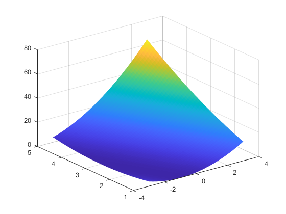
surf(x, y, z)
Produce figure for within the interval of
and
.
x = -3: 0.1 :3;
      y = 1: 0.1 :5;
      [X, Y] = meshgrid(x, y) % Produce a matrix for x and y

      Z = (X + Y).^2
      surf(X, Y, Z)
      shading flat
Mesh(x, y, z)
x = -3: 0.1 :3;
      y = 1: 0.1 :5;
      [X, Y] = meshgrid(x, y) % Produce a matrix for x and y

      Z = (X + Y).^2
      mesh(X, Y, Z)
Plot processing
Notations and control of axis
After producing the figure, you may need to note the figure.
| Command | Meaning |
|---|---|
| xlabel(string) | Name the x axis |
| ylabel(string) | Name the y axis |
| xlabel(string) | Name the x axis |
| zlabel(string) | Name the z axis |
| title(string) | Add the title on the top of the figure |
To control the axis, we can use the following commands
| Command | Meaning | Command | Meaning |
|---|---|---|---|
| axis auto | Set MATLAB to its default behavior of computing the current axes' limits automatically | axis manual | Freeze the scaling at the current limit |
| axis image | Same as axis equal except that the plot box fits tightly around the data | axis off | Turn off all axis lines, tick marks, and labels |
| axis on | Turn on all axis lines, tick marks, and labels | axis normal | Utomatically adjust the aspect ratio of the axes |
| axis ij | Place the coordinate system origin in the upper-left corner | axis xy | Draw the graph in the default Cartesian axes format with the coordinate system origin in the lower-left corner |
Axis(xmin xmax ymin ymax zmin zmax) % set the minium and maxium value for x, y and z axis
      Axis auto % set the value of axis as default

      Here is an example to control the axis for the plot of cos(1/x):

      ```matlab
      x = linspace(0.0001, 0.01, 1000)
      y = cos(1 ./ x)
      plot(x, y)
      axis([0.005 0.01, -1 1])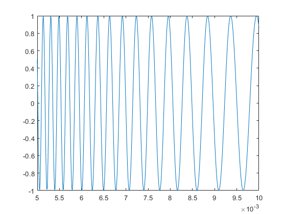
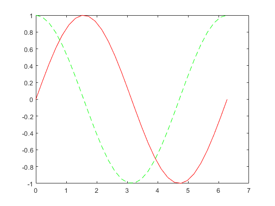
Combine figures
We sometimes need to combien different figures together. To do this, we use commands hold on and hold off. hold on retains plots in the current axes so that new plots added to the axes do not delete existing plots. hold off sets the hold state to off so that new plots added to the axes clear existing plots and reset all axes properties.
x = linspace(-pi,pi);
      y1 = sin(x);
      plot(x,y1)

      hold on;
      y2 = cos(x);
      plot(x,y2)
      hold off

      y3 = sin(2*x);
      plot(x,y3)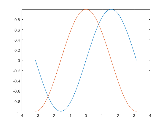
The style of line and color
We can also change the line into different styles and colors.
The stype of line
| Sign | `-` | `:` | `-.` | `--` |
|---|---|---|---|---|
| Meaning | Solid line | Dotted line | Dash-dot line | Dashed line |
The color of line
| Sign | `b` | `g` | `r` | `c` | `m` | `y` | `k` | `w` |
|---|---|---|---|---|---|---|---|---|
| Meaning | Blue | Green | Red | Cyan | Magenta | Yellow | Black | White |
The style of dot
| Command | Meaning | Command | Meaning |
|---|---|---|---|
| `.` | Point | `d` | Diamond |
| `_` | Line | `h` | Six-pointed star (hexagram) |
| `*` | Asterisk | `o` | Circle |
| `^` | Upward-pointing triangle | `p` | Five-pointed star (pentagram) |
| `<` | Left-pointing triangle | `+` | Plus sign |
| `>` | Right-pointing triangle | `x` | Cross |
| `v` | Downward-pointing triangle | `s` | Square |
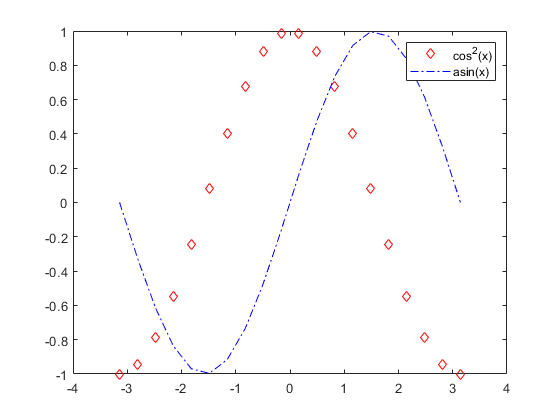
Grid, box and legend
grid is for displaying or hiding axes grid lines. box is for displaying or hiding axes outline. legend is for adding legend to axes.
grid on
      % displays the major grid lines for the current axes or chart

      grid off
      % removes all grid lines from the current axes or chart

      box on
      % displays the box outline around the current axes by setting their Box property to 'on'

      box off
      % removes the box outline around the current axes by setting their Box property to 'off'

      legend('string1', 'string2',...)
Here is an example to show how the legend can be added to the plot of two functions.
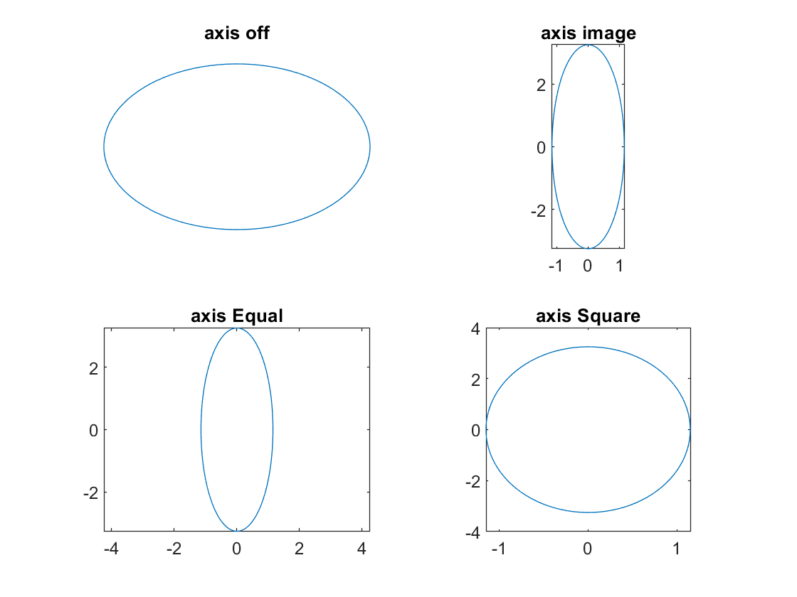
Subfigures
subplot(m,n,p) divides the current figure into an m-by-n grid and creates axes in the position specified by p. MATLAB® numbers subplot positions by row. The first subplot is the first column of the first row, the second subplot is the second column of the first row, and so on. If axes exist in the specified position, then this command makes the axes the current axes.
Here is an example to show how four ovals can be produced in one figure.
      t = 0:2*pi/99:2*pi;
      x=1.15*cos(t); y=3.25*sin(t);
      subplot(2,2,1); plot(x, y);
      axis off
      title('axis off');
      subplot(2,2,2); plot(x,y);
      axis image;
      title('axis image');
      subplot(2,2,3); plot(x,y);
      axis equal;
      title('axis Equal');
      subplot(2,2,4); plot(x,y);
      axis square;
      title('axis Square');